Data Methodology

by Léopold Salzenstein and Zander Venter (Norwegian Institute for Nature Research), and edited by Hazel Sheffield.

Introduction

In January 2024, the Norwegian public broadcaster NRK published a staggering investigation called “Norway in red, white and grey”. For the first time, in stark colours, Norwegians could see for themselves how much nature had been lost to the encroachment of motorways, cabins, business parks, and other developments in the country in a five-year period.

The investigation was the first of its kind, using artificial intelligence and satellite imagery to map “land take” – expansions of artificial surfaces over previously unbuilt areas – across Norway. Journalists from NRK worked in collaboration with Zander Venter, a leading expert in nature mapping from the Norwegian Institute for Nature Research, to acquire 40,000 satellite images of Norway. They used AI – manually fact-checked by the journalists – to analyse the images, looking for green areas that had been built upon between 2017 and 2022. Out came a map of Norway full of spots, each showing a small piece of destroyed nature.

Inspired by NRK’s investigation, Arena for Journalism in Europe, a non-profit supporting collaborative, investigative journalism – along with NRK – invited a group of European journalists to discuss expanding the methodology to the whole of Europe. In January 2025, an eleven-country team assembled from some of the continent’s foremost newsrooms began verifying thousands of satellite images and collecting stories of what has been lost. We published our findings in October 2025.

Here’s how we did it.

Key findings

European countries are converting significantly larger areas than previously estimated to residential housing, tourism resorts, industrial zones, and other types of development. While European biodiversity keeps declining at an alarming rate, countries kept sacrificing nature and farmland between January 2018 and December 2023, contrary to EU goals of reaching no net land take by 2050.
The investigation estimates that approximately 9000 km² of nature (~ 60%) or cropland (~ 40%) areas were replaced by built-up surfaces between 2018 and 2023 in Europe. This represents a rate of 1500km² of nature or cropland replaced by buildings every year – nearly double the interim target of 800km² every year, which was set by the EEA for the period 2000-2020.
According to an analysis conducted by the Norwegian Institute for Nature Research (NINA), four in every five instances of land take happened in already transformed ecosystems, including urban green spaces and semi-natural areas, such as pastures. Roughly two in every five instances of land take were due to the construction of residential areas, while one out of five instances of land take related to the construction of new roads and logistics centers.
We found more than 150,000 instances of land take overlapping with protected areas between 2018 and 2023 – more than 70 every day. Importantly, construction is sometimes allowed in so-called "protected" areas.
The analysis uses a new methodology to document recent land take in Europe. While the EU's environmental agency (EEA) provides data on land take up to 2018, our analysis covers developments all the way up to 2023 and is based on satellite images of higher resolution, also including small-scale land take and changes in urban green spaces for the first time.
Our investigation also finds that previous satellite-based estimates (most notably those of EEA) likely under-estimate the amount of land take in Europe, as they exclude changes that are smaller than 50,000m² (~five football fields) as well as changes in urban green spaces. In addition, the EEA methodology does not clearly account for the inaccuracies inherent to satellite-based land-cover estimates of land take. Contacted by Arena for Journalism in Europe, the EEA confirmed that its indicators likely under-estimate the amount of land take in Europe, “as has been shown when comparing with similar national indicators”. The EEA also said they were aware that their methodology “does not completely meet the requirements of statistical robustness”.

Mapping land take across Europe

Our initial step involved producing a Europe-wide dataset of land take, defined as the expansion of artificial surfaces over previously unbuilt areas.

Using a deep-learning model

We used Dynamic World, a land use and land cover dataset produced by Google and the World Resources Institute, employing a deep learning model.

The Dynamic World model uses 10-by-10 metre resolution satellite images from the two satellites of the Copernicus Sentinel-2 mission. It feeds these images to a fully convolutional neural network (FCNN), a deep learning image recognition model that categorises each pixel into one of nine land-cover classes.

The model, which is trained on global reference land-use and land-cover datasets, also assigns a class probability score – the probability of a pixel being one class or the other at a given time – to each pixel.

More information on Dynamic World is available here.

Algorithm tuning

To identify land take across Europe, we needed to isolate every pixel that changed from not being built-up to being built-up (something we describe as “built-up expansion”, or “land take”) between 2018 and 2023. Using the LUCAS A00 Artificial Land description, we defined "built-up" as an area characterised by artificial and often impermeable construction materials. This includes roofed and non-roofed construction, such as car parks and yards. It also includes linear features such as roads, as well as other artificial areas such as bridges and viaducts, mobile homes, solar panels, power plants, electrical substations, pipelines, water sewage plants, open dumps, greenhouses, and more. Land cleared for development was considered built-up unless it was re-vegetated by 2023 (e.g. planted with grass or trees).

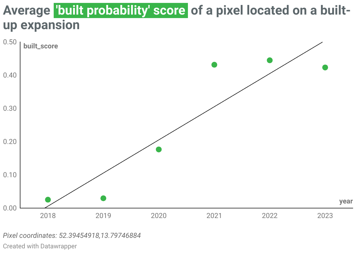
Our approach, designed by senior research scientist Zander Venter from the Norwegian Institute for Nature Research (NINA), involved fitting a linear regression through the built-up probability scores produced by the Dynamic World model for each pixel. Every pixel with a linear trend above a predefined threshold would be considered “built-up”.

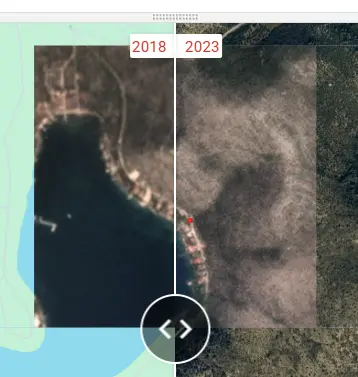
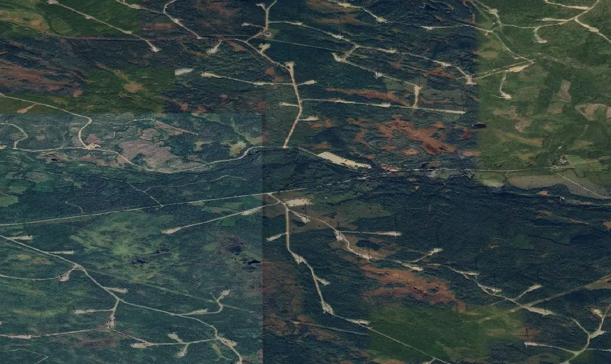
To illustrate this process, let’s take the example of a 10-by-10 metre area located in the municipality of Grünheide (Mark) in Brandenburg, Germany (coordinates 52.39454918, 13.79746884). As seen in Sentinel 2 satellite images below, this forested area was transformed into a factory in 2020. The “built probability” score allocated to this pixel by the Dynamic World model increased from 2018 to 2023, leading to a positive linear trend. This pixel was therefore classified as a “land take”.

Overall, we performed this analysis on approximately 84 billion pixels across Europe. To do this, we processed close to 185,000 Dynamic World images.

A GIF of a pixel on an area being built over time. — Pixel coordinates: 52.39454918, 13.79746884

Before running the analysis, however, we had to answer four questions:

How many years of satellite images should we feed to the model – and which ones?
What are the best months of the year for running the analysis?
What type of land-cover change should we consider when looking for land take?
What is the best threshold for accurately characterising a change from not built-up to built-up land cover?

Period of analysis

The Dynamic World data covers the period from June 2015 to the present day. However, our period of analysis only includes the years 2018 to 2023.

There are two justifications for this choice:

Dynamic World relies on satellite images from Copernicus’ Sentinel 2 mission. Until 2017, there was only one Sentinel 2 satellite circling the Earth, taking 10-by-10 metre resolution images of land and coastal zones once every 10 days. On March 7, 2017, a second Sentinel-2 satellite was launched, reducing the return rate to five days and increasing the amount of images taken every year. To increase the accuracy of our model, which depends on frequent imagery, particularly in regions with lots of cloud cover, we decided to start our analysis on January 1, 2018.
In order to verify the accuracy of the model, we needed access to good-quality reference material, or high-resolution aerial and satellite images of Europe. While a few European countries offer recent, high-resolution aerial imagery free of charge, most do not. We therefore had to rely on private providers such as Google Earth Pro. The images from these providers tend to be less frequently updated. To make sure that we could rely on high-resolution images during the verification process, we therefore excluded the most recent years (2024 and 2025) from the analysis.

In addition, the 2018 baseline year aligns with the production cycle of the EEA and Copernicus Land Monitoring Services. In particular, the Corine Land Cover backbone (CLC+) 2018, which matches the spatial resolution of Dynamic World, allowed us to disaggregate our results between cropland and nature areas.

Clearest months of the year

Because the Dynamic World model is run on images taken throughout the year, seasonal or weather variations – such as snow, tides, or clouds – can generate noise in the data. To reduce this noise, we decided to run our analysis only on the months of the year when the weather is the clearest and there is less “noise” in the satellite images.

These, however, differ significantly across Europe: in winter months, for example, results tend to be clearer in southern Europe, but snow and clouds tend to generate noise in northern Europe. During the summer months, droughts in southern countries also impacted the accuracy of the model.

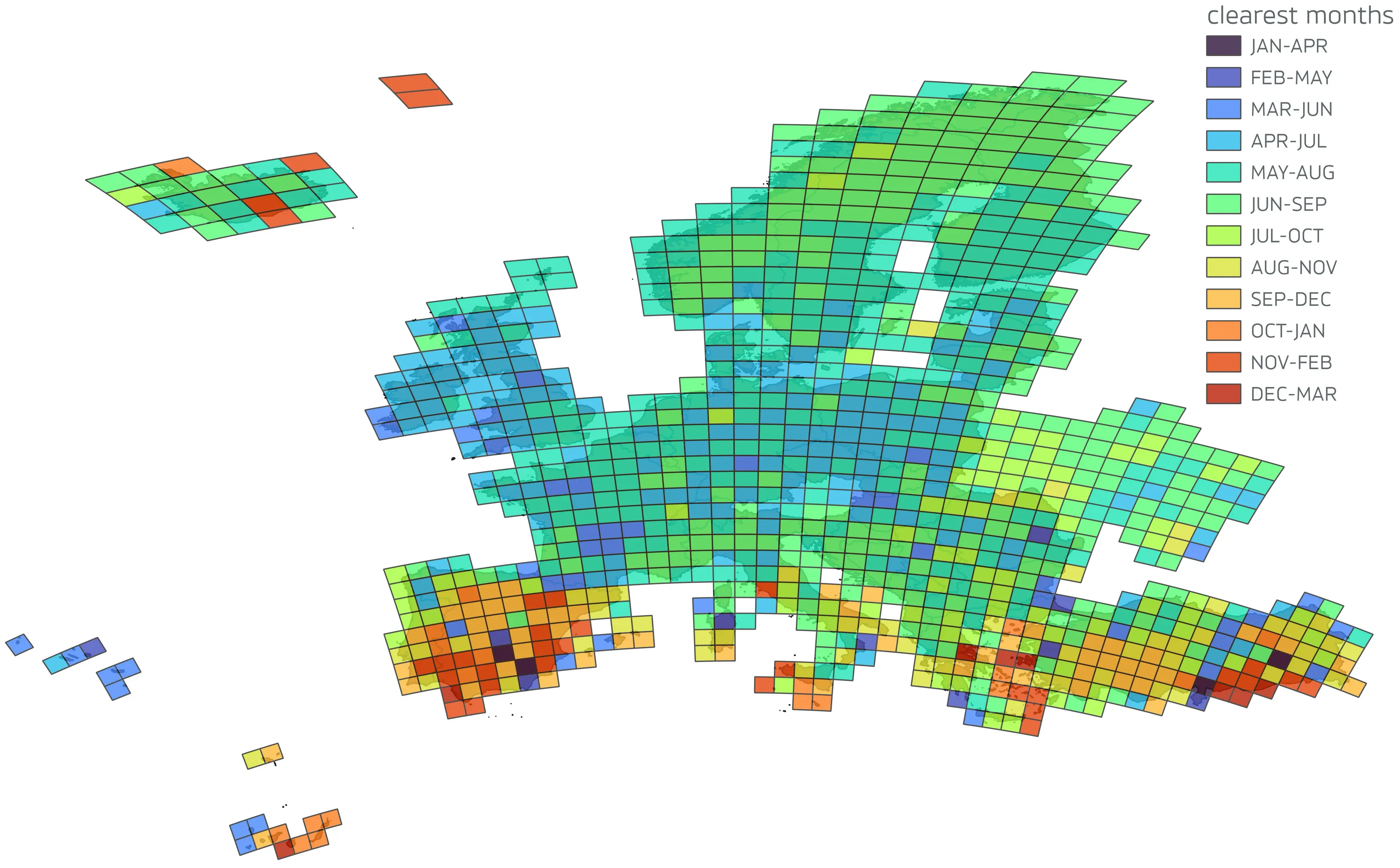
To find the clearest months of the year across Europe, we divided all of Europe’s land into a grid with a cell size of 100 x 100km. In each grid cell, we identified the four-month period in the year with the highest Dynamic World probability scores for the “built” class, using 30 random points located on built surfaces. We used the WorldCover 2021 map to isolate built surfaces, because it is shown to have higher thematic accuracy over Europe than Dynamic World or other global land cover maps. We could not use WorldCover to map land take because it is only produced for 2020 and 2021.

Based on this analysis, we then ran the model on the clearest four-month period for each 100 by 100 km area across Europe.

A map of Europe showing the clearest months period on a 100km x 100km grid. — Clearest months of the year for each 100x100km² grid cell over Europe

Land-cover classes

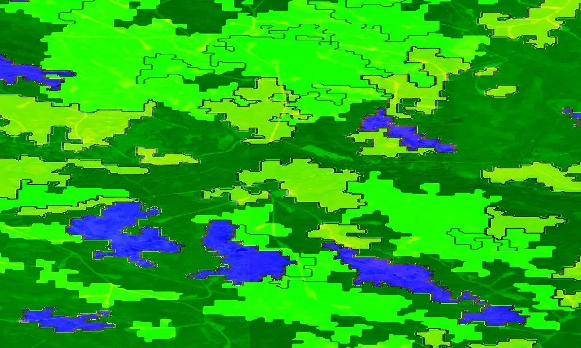
The Dynamic World model classifies each pixel into one of nine land cover classes: water, trees, grass, crops, shrub and scrub, flooded vegetation, built-up area, and bare ground.

To identify land take, we separated these classes into two groups: built-up and non-built-up.

This proved straightforward for eight of the nine land cover classes:

built-up includes Dynamic World’s built-up area class.
not-built-up includes Dynamic World’s water, trees, grass, shrub and scrub, crops, and flooded vegetation classes.

However, classifying Dynamic World’s “bare ground” class was more difficult. Indeed, this class can cover rocks and mountains, but also recently cleared construction sites. To overcome this issue, we ran two different versions of the model, one that only looked at the areas converted to “built-up area” and another one that considered both the areas converted to “built-up area” and “bare ground” classes. After the verification process, we found that the first version (built class only) of the model provided more accurate, less biased results – although estimates derived from pixel counting were much more conservative, especially in Nordic countries. When reporting country and EU-wide unbiased land take area estimates, we therefore relied on the first version of the model (built class only).

That said, each model tended to spot different types of built-up expansions: the former, more conservative model proved better at identifying finished building sites, while the second, more permissive model was better at finding sites under construction. To maximise our chances of finding relevant case studies, we decided to use both versions of the dataset in the second phase of the investigation – see sections below.

Linear trend threshold

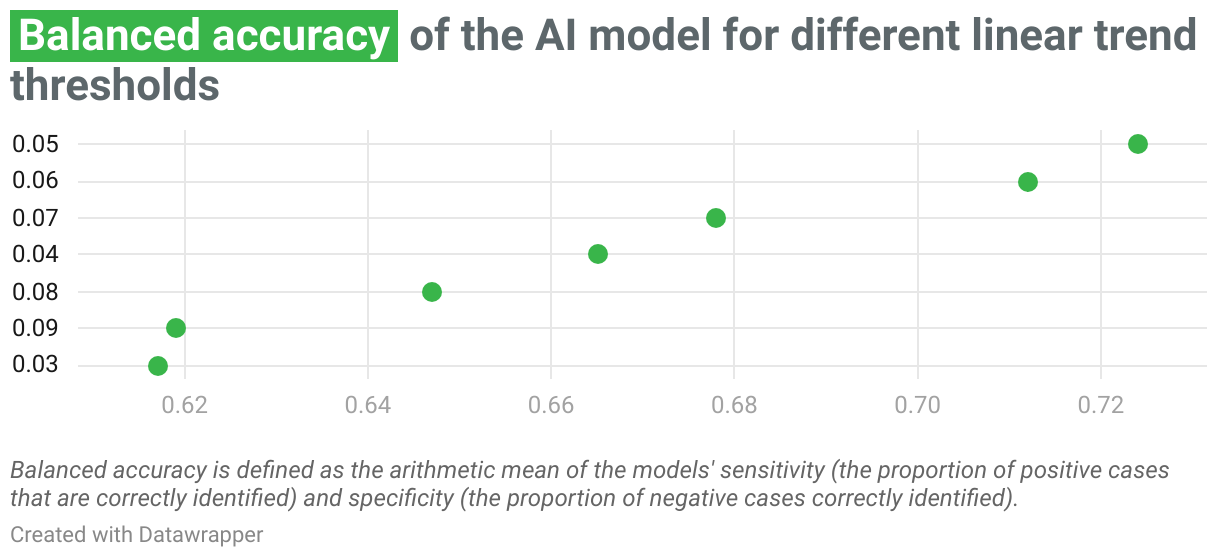
To identify the threshold above which a linear trend was most likely to accurately characterise a change from not built-up to built-up land cover, we produced a map of linear trends in built-up probability scores over Europe between 2018 and 2023, using images from June, July, and August.

Before officially starting the project, journalists at Arena for Journalism in Europe manually verified more than a thousand locations against high-resolution satellite images, such as those available on Google Earth Pro or the ESRI platform. The locations were chosen by randomly allocating points within land take pixels identified using a low threshold of 0.03.

By comparing the results of this manual verification with the map of linear trends in built-up probability scores, we found that a linear trend threshold of 0.05 provided the most accurate results across Europe. We therefore used this threshold to produce the final map.

Model output

After this initial phase of algorithmic tuning, we had two iterations of the model:

The first iteration identifies areas initially classified as nature or bare land by the model, and later classified as built-up.
The second iteration identifies areas initially classified as nature or bare land by the model, and later identified as either built up (from nature or bare land) or bare land (from nature).

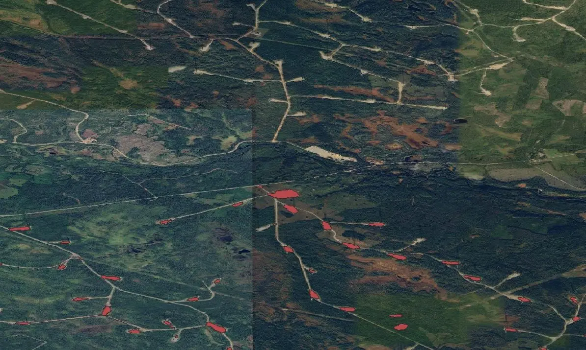
The two iterations of the model respectively identified approximately 2.2 and 2.6 million unique land take in 34 countries across Europe. Importantly, however, the number of land take is somewhat arbitrary because there is no clear definition of a singular land take. The mapping workflow we used converts connected pixels of land take into vector polygons.

These are what we refer to when we report the number of land take instances. A better way of quantifying land take is by estimating its area, which is the key indicator that we used. In countries where the model’s accuracy was high, land take instances were very useful for finding case studies, as discussed in the last section of this report. In other cases – most notably Spain, Greece and Italy – the lower accuracy of the model (see section “Accuracy of the model” below) meant that reporters had to use other strategies for finding relevant case studies.

To allow for more granular geographic analysis, we associated each identified land take polygon in the EU with its relevant Nomenclature of Territorial Units for Statistics (NUTS), level 2 and 3.

While our initial map showed land take across Europe, it did not distinguish between land take on cropland versus land take on nature. To isolate built-up expansion on land that was classified as natural in 2018, we used the Corine Land Cover backbone (CLC+) from 2018, because CLC+ was mapped at the exact same spatial resolution (10x10m) as our land take analysis. We isolated land take that took place on CLC+ pixels classified as anything other than cropland or built-up in 2018 (i.e. natural land cover). Then we broke down the natural land cover classes into grassland/wetland, shrubland, forest, and bare land. CLC+ does not cover Ukraine. Therefore, we extended a similar map called ELC10 over Ukraine. ELC10 contains the same typology and minimum mapping unit as CLC+.

Quantifying land take (2018-2023)

To estimate the amount of land taken across Europe, we decided against simply adding up the area of all the pixels identified by our model as being built-up expansion – a method called pixel counting. We knew that misclassification by the AI model was virtually inevitable and that simply counting the pixels would create biased area estimates.

Instead, we applied a scientific method called design-based area estimation, which allowed us to quantify the accuracy of our map and produce unbiased results associated with a 95% confidence interval. This does not mean there is a 95% chance the true area is in that range, but instead that, should we repeat the sampling and estimation process 100 times, about 95% of those confidence intervals would contain the true area.

We delimited the verification area as the thirty countries in the European Economic Area (EEA-30) plus Switzerland, Turkey, the United Kingdom and Ukraine, but then excluded Lichtenstein, Luxembourg, Cyprus and Malta due to resource constraints. These four countries are smaller than 10,000km² and therefore would receive a disproportionate verification effort. Country-level figures were therefore calculated for Austria, Belgium, Bulgaria, Czechia, Croatia, Denmark, Estonia, Finland, France, Germany, Greece, Hungary, Iceland, Ireland, Italy, Latvia, Lithuania, Netherlands, Norway, Poland, Portugal, Romania, Slovakia, Slovenia, Spain, Sweden, Switzerland, Turkey, Ukraine and the United Kingdom.

To be comparable with other European-wide estimates, we also calculated land take figures for the entire EEA-39 area - which also includes six cooperating Western Balkan countries (Albania, Bosnia and Herzegovina, Kosovo, Montenegro, North Macedonia, and Serbia). The countries we verified covered 96% of the EEA-39 land area and were therefore considered representative of the area as a whole.

Design-based area estimation

Here’s how we did it:

First, we split our Dynamic World map into different zones (strata). For example, one strata might be areas mapped as land take, another area mapped as stable land cover, etc. Strata represent zones for which we wanted area estimates.

Within each zone, we selected a number of random spots to check manually. We used high-resolution satellite images to view and classify each one of these spots. The goal was to create a reference dataset that was more accurate than the original map.

We then compared the actual result at each spot (land cover, whether the land was built on, etc.) with the map’s classification. We created a table, called an error matrix, to show where the map was correct and where it was wrong. Based on this error matrix, we then adjusted the initial land take estimates and computed a confidence interval, or a range within which the actual area was likely to fall, given the accuracy of the data.

In our case, we split the initial iteration of the map into 28 x 4 strata representing the 28 countries included in the analysis and the four mapped classes: land take on nature, land take on cropland, stable nature, and stable built/cropland.

You can find more detailed explanations of the design-based area estimation method here and here. Next, we provide more details on the different stages of the estimation process.

Data verification

Verification process

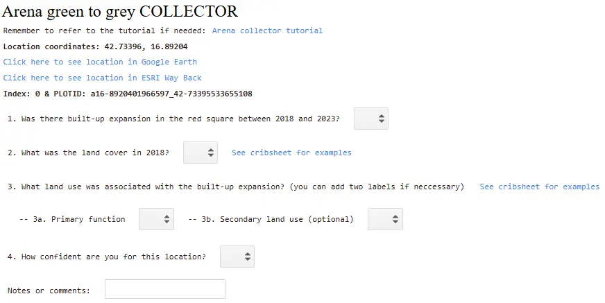
Forty journalists and fact-checkers manually verified more than 10,000 locations across Europe, a process that took more than 500 hours in total. As part of this process, journalists used high-resolution reference imagery from Planet Labs, Google Earth Online, and ESRI Way Back to manually classify each location.

For each point, journalists were asked to identify: (1) the land use land cover category in 2018; (2) whether land take took place between 2018 and 2023; and (3) when relevant, what type of built-up expansion took place (i.e. residential, industrial, etc).

When high-resolution imagery was unavailable for 2018 or 2023, journalists instead used PlanetScope satellite imagery, which provides 3-metre resolution imagery that is sufficient to identify land take. When relevant, journalists also used Street View websites to cross-check their assessment.

Journalists were given access to a bespoke web app facilitating and standardising this process. We used the responses to the first and second questions to compute the unbiased area estimate for land take, cropland loss and nature loss in each country. The answers to the last question served to assess the main drivers of land take in the EEA-39 area.

A screenshot of the app used by journalists to verify points.

Ensuring accurate verification

We adopted several measures to ensure an accurate and comparable verification process:

Before having access to the app, each journalist received training to understand and identify different land-use types in satellite images, as well as how to recognise land take and different drivers of loss in the region;
Journalists were randomly allocated points across Europe, regardless of their country of residence or their media outlet. Journalists also did not know how each point had been classified by the AI model, ensuring a blindfold verification process.
Journalists were asked to associate one of four levels of confidence with their verification. Points marked “uncertain” or “very uncertain” were separately double-checked by GIS experts from NINA or journalists at NRK and Arena. Points that remained “uncertain” or “very uncertain” after the expert review were excluded from the analysis.
Similarly, points marked as either false positives or false negatives were separately double-checked by GIS experts from NINA or journalists at NRK and Arena.
To ensure accurate classification, journalists were given access to a reference images library of different types of land use and land cover classes across Europe. To do this, we used the LUCAS survey’s typology, which classifies specific areas based on in-situ visits and is therefore considered ground truth. Using this reference library, verifiers could easily check, for example, what a forest looks like on satellite images in any specific part of Europe. This was important, as forest or grassland, for example, may look very different in northern and southern Europe.
Verifiers were also given access to a reference images library of nature loss drivers (i.e., residential, mining, transport, industry, etc.), also derived from the LUCAS survey, which maps both land cover and land use. Land use drivers were classified according to LUCAS typology, which includes primary, secondary and tertiary land use industries.

Accuracy of the model

As mentioned above, we used a scientific method called design-based area estimation to quantify the accuracy of our map and correct the area estimate associated with each class.

Using this method, we calculated the overall accuracy (oa) of the map, as well as the user accuracy (ua) and producer accuracy (pa) of each class within the map (i.e. stable nature, stable cropland, land take, etc.), by country:

Overall accuracy is a general measure of how well our map matches the real world. It tells us the proportion of all the pixels that were correctly classified across all the categories.

The overall accuracy is calculated by summing the individual class accuracies, using the equation

O A = \sum_{j = 1}^{q} P_{j j}

, where $P_{j j}$ is the proportion of correctly mapped samples for class $j$ and $q$ is the total number of classes.

User accuracy is a measure of the reliability of the map for a specific class. For example, a high user accuracy for the class ‘land take’ means that the map has few areas wrongly classified by the model as land take, or ‘false positives’.

The user accuracy is calculated by measuring the proportion of the area mapped by the model as class $i$ that was correctly classified as class $i$ , using the equation $U A = \frac{P_{i i}}{{P .}_{r}}$ , where $P_{i i}$ is the proportion of samples that were truly class $i$ and classified as class $i$ , and $P_{. i}$ is the proportion of samples classified as class $i$ .

Producer accuracy measures how complete the map is for a specific class. For example, a high producer accuracy for the class ‘land take’ means that there are few instances of land take that the model did not classify as such, or ‘false negatives’.

The producer accuracy is calculated by measuring the proportion of the area of the reference class $j$ that was correctly mapped as class $j$ , using the equation $P A = \frac{P_{j j}}{P j .}$ , where $P_{j j}$ is the proportion of samples that were truly class $j$ and classified as class $j$ ; and $P_{j .}$ is the proportion of samples that truly belong to class $j$ .

Here is a breakdown of the overall accuracy of the map, as well as the user accuracy and producer accuracy for the ‘land take’ class, by country.

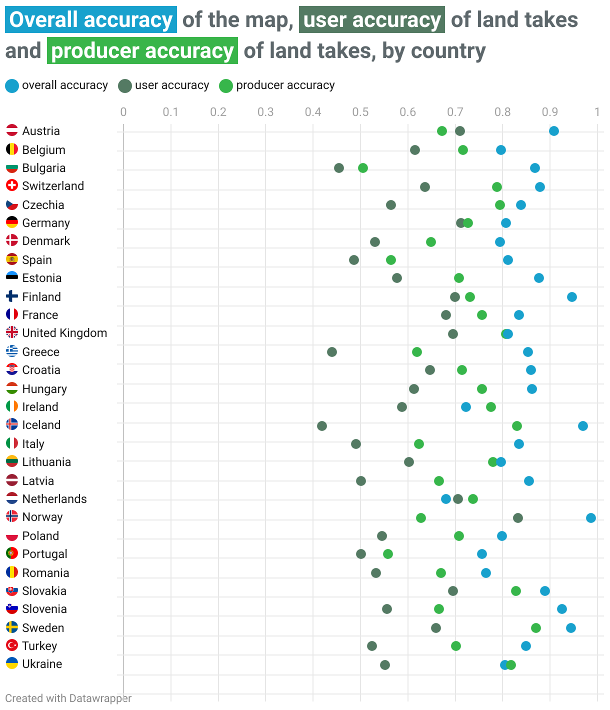
The proportion of false positives and false negatives varied sometimes significantly from country to country. Overall, southern European countries such as Greece, Spain and Italy – as well as Iceland - had a higher proportion of false positives compared to northern European countries. This also impacted the overall accuracy of the model in these countries.

To account for and correct for these differences of accuracy, we then computed an unbiased area estimate – a statistically robust assessment of the area of nature or cropland that was destroyed due to new constructions in each country.

To do this, we first calculated the stratified estimator of the proportion of area for class $k$ , using the following equation from Olofsson et al 2014:

p_{k} = \sum_{i = 1}^{q} W_{i} (\frac{n_{i k}}{n})

Where $p_{k}$ is the stratified estimator of the proportion of area for class $k$ ; $W_{i}$ is the known area proportion of map class $i$ ; $n_{i k}$ is the sample count at cell $(i, k)$ in the error matrix; and $n_{i}$ is the total sample size for map class $i$ .

We then estimated the unbiased area estimate of each class $k$ , using the equation $A k = A \times p_{k}$ , where $A_{k}$ is the estimated area of class $k$ , $A$ is the total map area, and $p_{k}$ is the stratified estimator of the proportion of area for class $k$ .

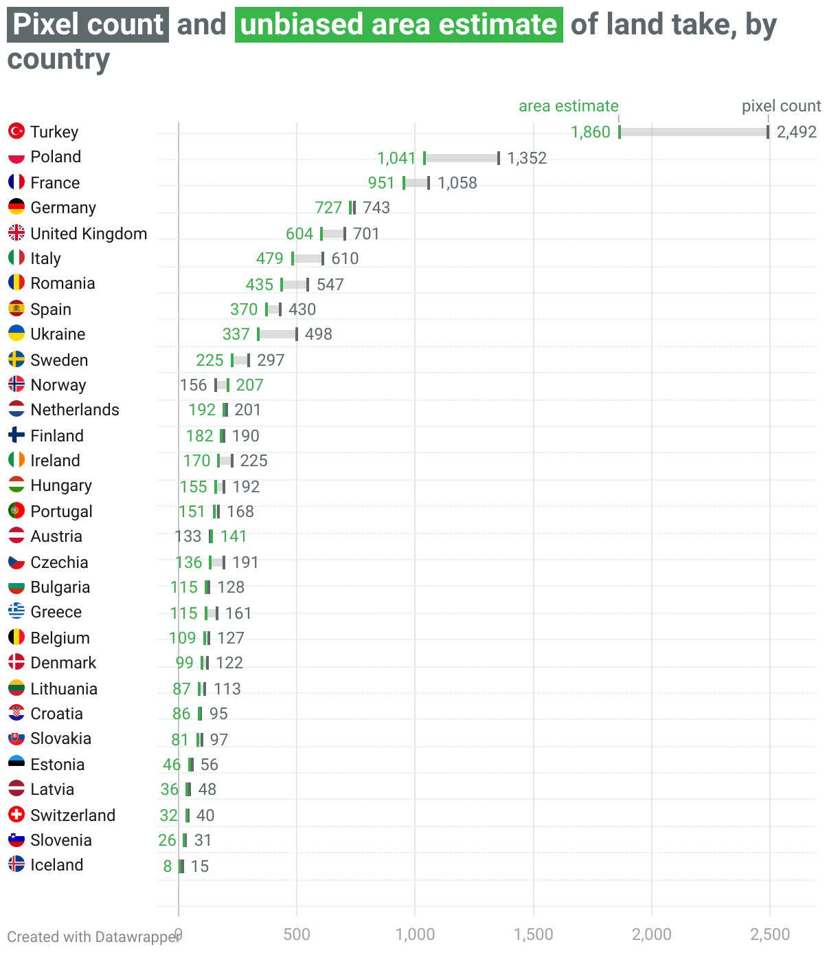
The graph below shows the difference, for each country, between the ‘biased’ area estimate obtained by summing all the pixels classified as ‘land take’ in the map, and the ‘unbiased’ area estimate calculated using the design-based area estimate method.

We also calculated a 95% confidence interval for each area estimate of the ‘land take’ class for each country.

To do this, we first estimated the standard error of the estimated proportion of each area, using the following equation from Olofsson et al 2014:

S (p_{. k}) = \sqrt{\sum_{i} W_{i}^{2} \frac{(\frac{n_{i k}}{n_{i}} (1 - \frac{n_{i k}}{n_{i}}))}{n_{i} - 1}}

Where $S (p_{. k})$ is the standard error of the proportion of area for class $k$ ; $W_{i}$ is the known area proportion of map class $i$ ; $n_{i k}$ is the sample count at cell $(i, k)$ in the error matrix; and $n_{i}$ is the total sample size for map class $i$ .

We then calculated the standard error of each unbiased area estimate $A_{k}$ , using the following equation: $S (A_{k}) = A \times S (p_{. k})$ Where $S (A_{k})$ is the standard error of each unbiased area estimate $A_{k}$ ; $A$ is the total map area and $S (p_{. k})$ is the standard error of the proportion of area for class $k$ .

Finally, we calculated the 95% confidence interval of each area estimate using the equation $C I (A_{k}) = A_{k} \pm (1.96 \times S (A_{k}))$ .

The unbiased area estimate and 95% confidence interval of the land take class in each country is presented in the next graph:

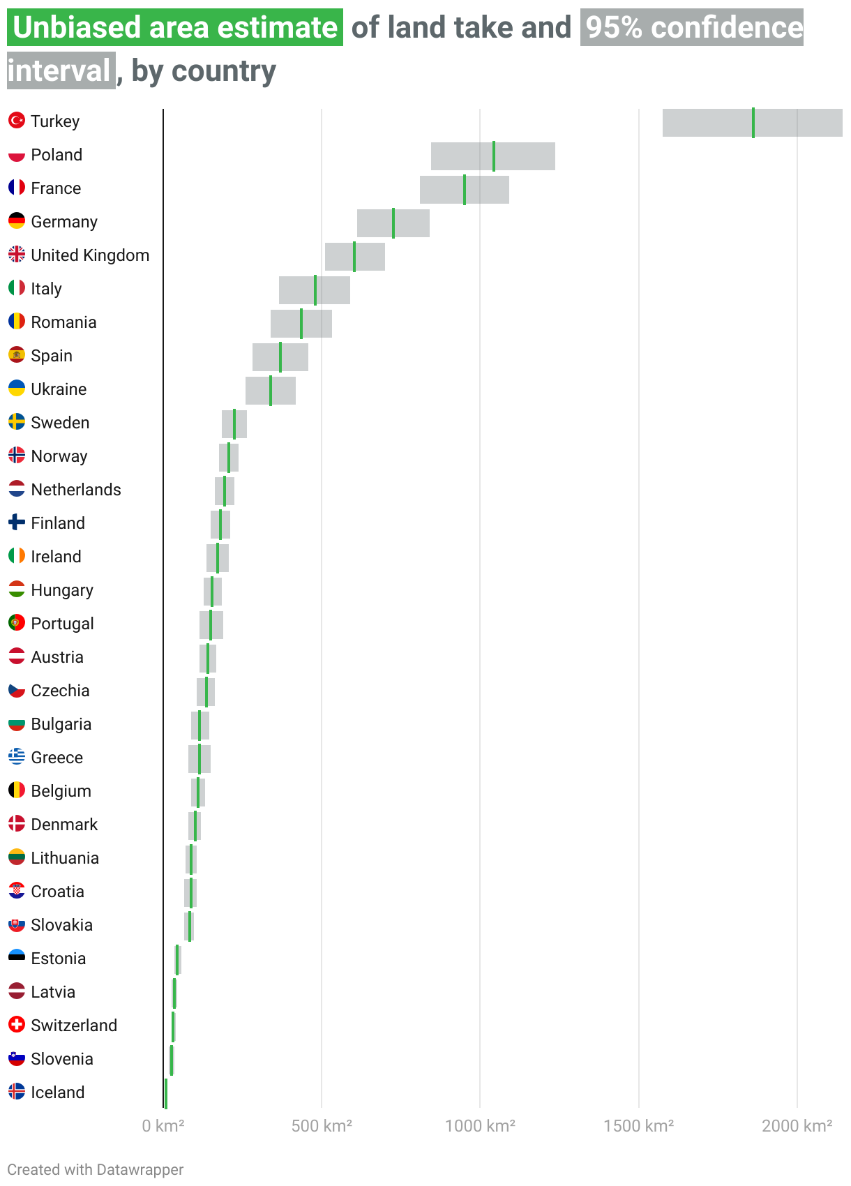
The unbiased area estimate for the EEA-39 was approximately 9000km², with a confidence interval of roughly 300km². When we divided this for the six years of our analysis, we obtained a yearly average land take of 1500km², with a 95% confidence interval of approximately 50km².

The code for the European analysis is freely available on Github.

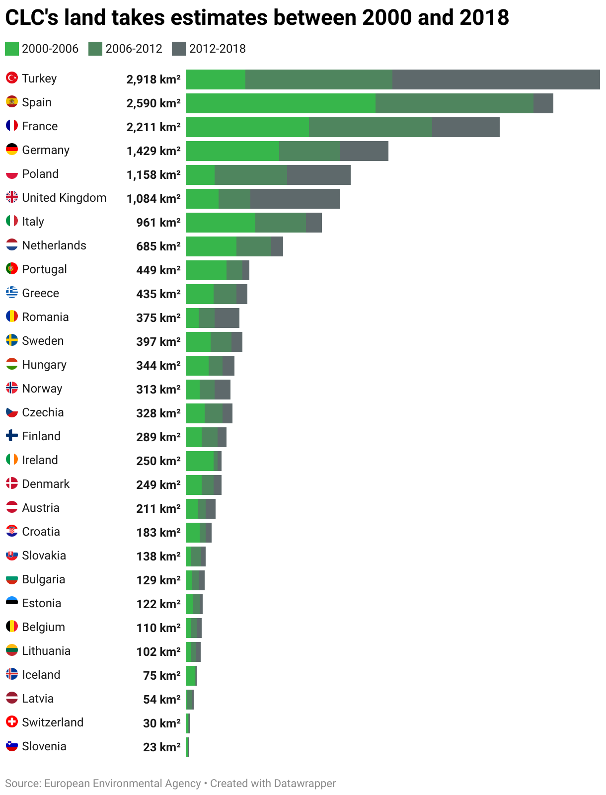
Quantifying pre-2018 land takes

In order to provide context for our 2018-2023 results, we conducted further analysis of European countries’ land take trend between 2000 and 2018. For this, we used the European Environment Agency’s calculation of land take statistics by country and ecosystem, which are based on Corine Land Cover Accounting Layers.

Corine Land Cover Accounting Layers

Corine Land Cover Accounting Layers are specialised geospatial datasets derived from the EU's Corine Land Cover program, which maps land use and land cover across Europe. They were created specifically to measure changes in land cover and ecosystems over time.

CLC accounting layers are created by combining the lower resolution CLC status layers (minimum mapping unit = 25ha) and the higher resolution CLC-change (CLCC) layers (minimum mapping unit = 5ha). They are fully comparable from 2000 onwards, allowing for time series analysis of three 6-year periods: 2000–2006, 2006–2012, and 2012–2018. CLC accounting layers for the next period (2018-2024) are scheduled to be released in mid-2026.

You can find a detailed discussion on the CLC accounting layer here.

Data differences

There are important methodological differences between our European dataset of land take and the Corine Land Cover Accounting Layers.

Whereas we use a 100m² minimum mapping unit (10x10m pixel), CLC accounting layers use a 50000m² minimum mapping unit. This means that there are significant differences between the two maps. Gardens, small forests, and road verges, for example, are mapped as nature in our map, but marked as built or artificial in CLC. Similarly, small land take areas, such as wind turbines or isolated houses, are likely too small to be identified as land take in CLC accounting layers. In addition, CLC only maps road construction or railways if they are at least 100m wide – only large motorway constructions are therefore included in the CLC map.

Comparison between our model and Corine Land Cover, using the example of a wind farm in Sweden. — Wind turbines built before and after 2018 in northern Sweden (coordinates: 65.342128, 20.8401016).

Finally, whereas our map considers all urban development on green spaces as land take, developments on green spaces within the boundaries of a settlement are not counted as a built-up expansion in the CLC accounting layers.

In their replies to Arena for Journalism in Europe, the EEA confirmed that their indicators likely underestimate the amount of land take in Europe, “as has been shown when comparing with similar national indicators” due to the fact they use a data source that cannot detect constructions smaller than 5 hectares.

Accuracy of CLC accounting layers

At the basis of CLC accounting layers is human and machine interpretation of satellite images. As a result, figures of land take reported by the EEA using CLC accounting layer are likely to include false positives and false negatives, just like our own data.

As mentioned above, our estimations of land take by country are purposefully corrected to account for the estimated accuracy of our model. By comparison, amounts of land take reported by the EEA simply represent the sum of all areas identified as land take in the CLC accounting layer, a process called pixel counting. In simple terms, this means that EEA figures do not account for potential inaccuracies in the CLC accounting layers.

Contacted by email, the EEA confirmed that they report “pixel counting” estimates, and said they were "aware that the methodology applied does not completely meet the requirements of statistical robustness”. The EEA said that there were “practical limitations” to reporting statistically corrected figures - partly because waiting for a complete validation of the data before publishing their results would likely generate further delays.

According to an independent validation report of the CLC 2018/CLC Change 2012-2018 layer, there are significant variations in the user accuracy and producer accuracy of CLC land take classes. Similar variations were also observed for the 2006-2012 period.

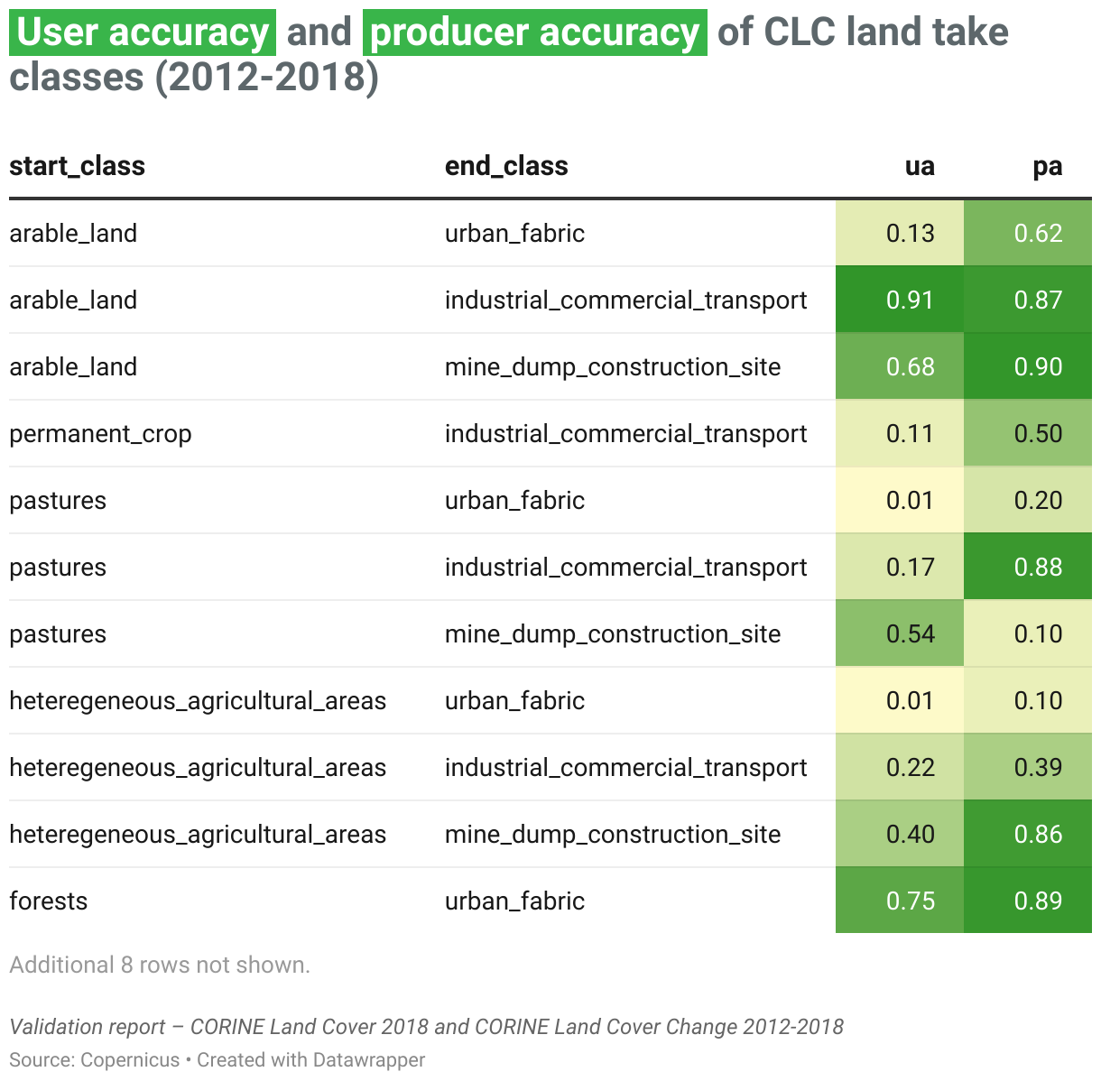
Unfortunately, user accuracy and producer accuracy of CLC’s land take classes are only available for the period 2006-2012 and 2012-2018. When contacted, the EEA could not provide us with the sample points used to verify the CLC accounting maps.

Accordingly, we were not able to compute unbiased area estimates and a 95% confidence interval for the EEA’s land take area estimate for the period 2000-2018. Instead, we rely on the pixel-counting estimates provided by the EEA. In its reply to our questions, the EEA said that it was following technical progress emerging from the scientific community to better use satellite images for tracking land change in the future.

Finding case studies

In parallel to conducting our data verification and analysis, we used the raw maps produced by the AI model to identify specific cases across Europe.

Cross-referencing land take with nature data

An initial step involved ranking all the land take areas from largest to smallest, by country. Each country team was provided with the largest identified land take in their country, as well as information about the land cover on which the building took place, as identified by the Corine Land Cover backbone (CLC+) in 2018.

For ease of use, the data was provided in various formats (CSV, Geopackage, and KLM), allowing journalists to identify building sites in areas identified by satellite analysis as being natural land (i.e. wetland, forest, etc.).

However, the CLC+ data does not separate different qualities of natural areas, for example, old-growth forest from a timber plantation. In order to identify areas built on top of truly valuable nature, we therefore cross-referenced the built-area map with geospatial datasets of valuable nature. This process involved finding overlaps between the polygons identified as built-up expansions by the AI model and polygons of various natural areas (forests, wetlands, grassland, etc). We conducted this process both at a European level, and using national-level data in partner countries.

The definition of what constitutes valuable nature varies greatly from context to context, as nature's value is dependent on who is doing the valuation and their philosophical and ethical standpoint. No matter the paradigm, the definition is fraught with contradictions. As a result, we purposefully did not provide a strict definition of “valuable nature”. Instead, each country team was able to select which type of nature to focus on, depending on their national context.

The cross-referencing process was conducted using QGIS and PostGIS.

A list of natural-area data at the European and national levels is available here.

Cross-referencing land take with protected areas

Sometimes, valuable nature is also given protected status under national, regional or local laws. Not all such protections prevent construction or urban development, meaning that constructing in a so-called “protected area” may still be legal. Nonetheless, we decided to calculate an estimate of land take in such areas, even where building is not prohibited, in part to see if it would reveal any interesting case studies. To do this, we cross-referenced our dataset with the World Database on Protected Areas (WDPA), a global database of terrestrial and marine protected areas.

We then selected and verified a random sample of 200 apparently overlapping polygons to measure the accuracy of our data. This allowed us to account for potential inaccuracies and correct our estimates. We then purposefully selected a conservative, rounded figure, which likely under-estimates the amount of land take in protected areas.

Case study: impact of tourism in Lapland

Arena for Journalism in Europe, The Guardian, Le Monde and the Finnish journalism platform Long Play also calculated the impact of tourism on one of the continent’s remaining pristine woodlands, that of Finnish Lapland.

The Lapland phase of the analysis took part in two stages:

First, we used a statistically generated sampling method, carrying out 400 checks on 1,800 developments captured by the algorithm - randomly selected but in keeping with the distribution of all detected polygons.

Each of the 400 polygons was manually checked to:

Ascertain the overall accuracy of the algorithm’s detection. When we included 'partial' developments as ‘accurate’, we estimated 76% user accuracy. When we excluded these points, we estimated 66.25% accuracy. The user accuracy of the wider Finland map was 70%, meaning that Finnish Lapland has a similar accuracy to the rest of Finland.
Record the development’s current land use (residential, logistic, etc). Where the development was for the purposes of tourism we further recorded the type of tourism activity (hotel, holiday rental, tourist recreation site, etc). We extrapolated from the 400-strong sample that an estimated 13.8% (plus 1.9% partially involved) of the correctly identified polygons were tourism-related.

Second, in order to calculate the scale of development in those areas that attract most tourists we concentrated on those areas with the highest number of bed-places per capita (Inari, Kittilä, Kolari, Enontekiö and Pelkosenniemi) as well as Rovaniemi, the regional capital which hosts an airport and "Santa Claus's village". Using tourism hot spots (as identified by local reporters) as our centre points (ski resorts, historical centers, etc) we extracted all polygons within a 10km radius of these centre points.

Where the AI model correctly identified a development, but over- or under-estimated its actual size, we manually redrew the polygon boundary using QGIS or Google Earth Pro. Any false positives (polygons where the AI incorrectly identified development) were excluded from the analysis. Conversely, some false negatives, developments not captured by the AI, were added to our data. Even when accounting for the addition of these false negatives we almost certainly have not identified all developments, therefore we consider our estimates to be conservative.

We then manually checked whether each polygon in these areas was for the purpose of tourism, cross-referencing each development against sources including Google Maps, Open Street Map, AirBnB and Booking.com.

Commercial services for tourists (such as husky farms, ski resorts, snow mobile rental sites, etc) were considered “touristic” for the purposes of this analysis whereas sites that offer recreational/commercial services to the local population (e.g. swimming pools, museums, gyms/service stations) were excluded.

Roads were included where the connected development was solely for tourism purposes. We excluded other constructions that were not directly related to tourism - although tourism was likely a secondary driver for some of them. Therefore, our analysis likely under-estimate the real impact of tourism in Finnish Lapland.

Limitations

European data sources that are based on satellite image analysis, such as the Corine Land Cover Accounting Layers, have some limitations when monitoring net land take. These databases are primarily land cover databases that analyse the surface of the Earth (i.e. artificial, forest, grassland, water, etc.), while land use databases instead use cadastral data to assess the way a specific surface is being used. This can lead to sometimes significant differences between European and national assessments of land take. This limitation also applies to our dataset of European land take between 2018 and 2023.

Similarly, as explained above, maps that are derived from the observation of satellite images are subject to potential errors or inaccuracies. As explained above, we have done our best to quantify and account for these inaccuracies in our own estimates of land take.

In addition, the accuracy of satellite-derived maps is highly dependent on the resolution of the input images. Since the Dynamic World model relies on 10m resolution satellite images, it may miss instances of land take that are smaller than 100m². As mentioned above, the CLC accounting layer does not take into account land take instances that are equal to or smaller than 50000m².

Another limitation stems from the availability of valuable nature datasets. Some of the countries included in the analysis had little to no national data on valuable nature. Sometimes, valuable nature had only been mapped before or after 2018, which could lead us to miss important built-up expansions over valuable nature.

Finally, we are aware that our project has its own environmental cost. To estimate the emissions resulting from generating our European map of land take, we sent an email to Google, asking about the energy use of its infrastructure. While no official answer from the company arrived in time for publication, a Google employee suggested we prompt an LLM to answer our question. While we were aware of the paradox of asking an AI to calculate this, we nonetheless fed our Google Earth Engine script to Gemini, Claude, and ChatGPT to assess our analysis’s likely environmental footprint. Because of the widely different estimates, we opted not to base our assumptions on those results. We welcome any reliable expertise and input to establish a more accurate figure and will update this section if Google provides an official reply.

Contributions by Anne Linn Kumano-Ensby (NRK), Mads Nyborg Støstad (NRK), Ruben Solvang (NRK), Bálint Czúcz (NINA), Trond Simensen (NINA), Zeynep Sentek (Arena), Jelena Prtoric (Arena), Hazel Sheffield (Arena), Raphaëlle Aubert (Le Monde), Pamela Duncan (The Guardian), Lotta Närhi (Long Play), Eurydice Bersi (Reporters United).